Constraints

Introduction

The Constraint Tool provides features for both analyzing and generating constraints for structure generation, and for assigning NOE spectra. The tool can take one or more peak lists and generate possible assignments for the peaks. A first step in the analysis displays the number of peaks that can be assigned, including a count of those with an excessive number of assignment possibilities. An iterative procedure can be used to automatically adjust the assignment tolerance to match a target fractional assignment.

Distance Constraint Table

The constraint table displays a large amount of information about structural constraints. These constraints can be generated internally, through manual peak assignment, the peak identification tool, or the peak extract and assign mode of the constraint table. They can also be read in from external sources such as XPLOR constraint files, ARIA XML restraints files. The values displayed here were obtained upon reading in a merged STAR file from the BMRB containing assignments, constraints and a family of conformers.

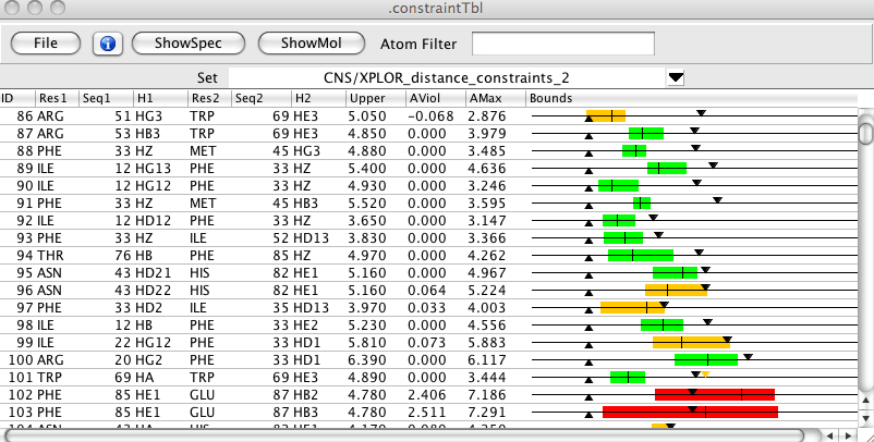
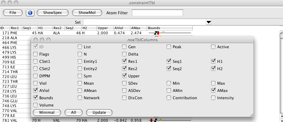
Over 35 different values can be displayed for constraints. These include the atomic assignments, the origin peak, chemical shift violations, whether cross diagonal peaks were found, upper and lower distance constraints, and various distances both for the specific constraint, and averaged over all the constraints assigned to a peak. In addition there are columns for a network anchoring contribution, a distance violation contribution, and a summary value indicating the probability for the particular assignment. Bounds are graphically displayed within the table. The total amount of information can be somewhat overwhelming, so it is possible to turn on and off the display of each column.

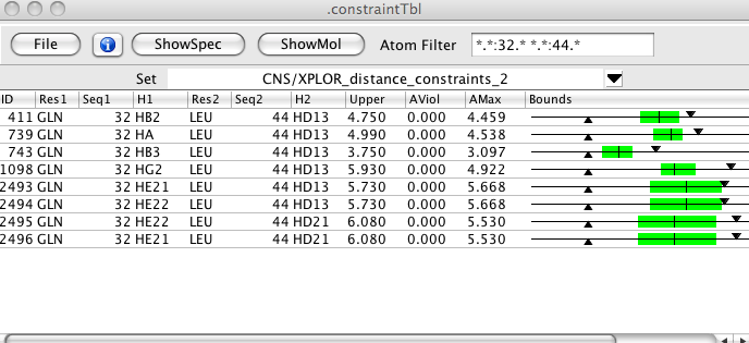
Filters can be set so that only constraints involving a single or pair of residues are displayed. This table is shown with a small set of columns, including the graphical bounds which illustrate the lower and upper bounds with triangles, the range of distances in the set of structures with a colored region, and the mean distance with a single vertical line. If bounds are violated the bound region is colored orange or red, depending on the violation.

ID

A unique numerical id for this constraint

List

The peak list this constraint came from

Gen

How was this constraint generated. See list below for descriptions.

Peak

The id number for the peak this constraint came from

Active

Is the constraint currently active

Flags

Character flags indicating reasons the constraint might be inactive. See list below for descriptions.

N

The number of possible assignments for the peak giving rise to this constraint.

Delta

The difference in residue numbers for the two atoms of this constraint.

CSet1

The coordset for atom 1 of this constraint.

Entity1

The entity for atom 1 of this constraint.

Res1

The residue name for atom 1 of this constraint.

Seq1

The sequential number for the residue of atom 1 of this constraint.

H1

The name of the atom (typically a hydrogen) for atom 1 of this constraint.

CSet2

The coordset for atom 2 of this constraint.

Entity2

The entity for atom 2 of this constraint.

Res2

The residue name for atom 1 of this constraint.

Seq2

The sequential number for the residue of atom 1 of this constraint.

H2

The name of the atom (typically a hydrogen) for atom 1 of this constraint.

DPPM

A number running from 0 to 1 representing a Gaussian function of the deviation between the chemical shifts of the peak and those of the assigned atoms. The higher the number the more likely the assignment.

Sym

Peak has a symmetry related (cross diagonal) peak with the same assignment as this constraint.

Upper

Upper Bound

Viol

The distance violation for the structure with the biggest violation.

Mean

The mean distance between these atoms.

SDev

The standard deviation of the distance between these atoms in all structures.

Min

The minimum distance between these atoms in all structures.

Max

The minimum distance between these atoms in all structures.

AViol

The distance violation for the structure with the biggest violation. Violation is averaged over all constraints from the originating peak. This value will be the same for all constraints from that peak.

AMean

The mean distance between these atoms. The distance is averaged over all constraints from the originating peak. This value will be the same for all constraints from that peak.

ASDev

The standard deviation of the distance between these atoms in all structures. The distance is averaged over all constraints from the originating peak. This value will be the same for all constraints from that peak.

AMin

The minimum distance between these atoms in all structures. The distance is averaged over all constraints from the originating peak. This value will be the same for all constraints from that peak.

AMax

The minimum distance between these atoms in all structures. The distance is averaged over all constraints from the originating peak. This value will be the same for all constraints from that peak.

Bounds

A graphical depiction of the constraint bounds. Downward pointing triangle is the upper bound. Upward pointing triangle is the lower bound. Colored bar indicates the range of distances in the set of structures. The vertical line in the bar is the average distance in the set of structures. The bar will be green if all structures are within the bounds, orange if some are outside the bounds, but the mean is withing the bounds, and red if the mean is outside the bounds. If the constraint is a short range one for which an analytical value for the maximum distance can be calculated this will be indicated as an orange triangle.

Network

Network constraint value. The more constraints there are, and the higher there contribution values are, between the residue pairs this constraint involves, the higher this value will be.

DisCon

If structures are present this is a measure of well the distances between the atoms fit with the distance bounds. The value ranges from 0 to 1 and 1 indicates that all structures have the distance within the bounds.

Contribution

A value that summarizes the contribution of this constraint to the possible assignments for this peak. The value runs from 0 to 1 and 1 is best.

Intensity

The intensity of the peak that this constraint is derived from.

Volume

The volume of the peak that this constraint is derived from.

Constraints can be derived in various ways and this is indicated in the Gen column of the table. The values that may be seen in the table are described here.

Auto

Constraint generated by the automated extract and assign procedure using the internal peak id code. If constraint list was read in from an ARIA XML file then this indicates the constraint was automatically generated by ARIA.

AutoP

Constraint generated by the automated extract and assign procedure using the internal peak id where at least one manually assigned constraint for the peak was present. code.

Semi

If the constraint list was read in from an ARIA XML file then this indicates that one of the dimensions of the constraint was automatically generated by ARIA and the other was from a manual assignment.

Man

Constraint generated from a specific assignment of the atoms of the peak.

Constraints can be marked as inactive based on various criteria. These criteria (and there may be more than one value for each constraint) are indicated in the Flag column of the table. The characters in the table have the following meanings.

r)edundant

There is more than one constraint between the same two atoms. This is one of the ones removed.

f)ixed

The distance between these atoms is fixed by the structure so this restraint is of no value.

a)mbiguous

There are more than the specified maximum number of constraint possibilities for this peak. That is, it is too ambiguous.

d)iagonal

The proton pairs for this constraint represent the same atom.

p)pm

The Gaussian function of the deviation of chemical shifts between the peak and the atom assignments is below the specified threshold.

v)iolation

The distance violation of this constraint in the current structures is too large.

u)user

Constraint inactivated by the user.

Generating Constraints from NOESY Peaks

The first step of generating constraints from one or more NOESY peak lists is to specify which lists are to be used, and check the tolerances and offsets of these peak lists. Select the <span class="menuchoice">File > Peaklists... menu item from the menu bar of the Constraint Table to get the interface shown.

Next, click the Add List button to add a new peak list row to the interface. Here we've added two rows and then selected an N15 Noesy for one row and the C13 NOESY for the other. The peak lists are selected with the pull down menu in the PeakList column. Constraints can be generated with values proportional to the peak volume or intensity. Select the value with the combobox in the MMode (for Measurement Mode) column.

Before continuing with extracting and identifying constraints from the peaks it's important to check the tolerances that will be used. Click the button in the Tolerance column to bring up the following interface. The values in the the fields directly under the peak dimension labels (HN, H1, and N) are the current peak identification tolerances for this peak list. The Assignability Statistics in the lower section of the interface is updated when you click the Update button (or execute various other functions in the interface). Each peak can be classified in one of three ways. Assignable Peaks are those whose chemical shifts are consistent (within the specified tolerances) of some assigned set of atoms in the molecule. If the peak is assignable, but there are more than the specified (with the MaxAmbig entry at top) possible assignments it is instead put in the MaxAmbig category. If the peak cannot be assigned it is in the Unassignable category. The number of peaks, and the fraction of the total number of peaks, is shown in the N and Fraction columns. Every time you click the Update button the software essentially simulates the assignment of the peak list to calculate these statistics.

If the tolerances are too tight, a large number of peaks will be unassignable, whereas if the tolerance is too loose, there will be too many possible assignments for the peaks, and the number of peaks in the MaxAmbig category will be high. A good starting point for the tolerances can be obtained by clicking the Guess button. This will set the tolerance to the median line width for the peaks in each dimension.

You can optimize the tolerances by clicking the Optimize button. This will iteratively modify the tolerances until the fraction of assignable peaks (Assignable + MaxAmbig)/nPeaks is close to the target value set with the slider. The tolerances for the different dimensions will be changed so that the ratio between the tolerances will be the same at the end of the optimization as they are at the beginning. To explicitly change that ratio for the starting point enter specific values into the tolerance fields.

The referencing of the peak list and the assigned atoms may be different depending on where the atom assignments came from. Clicking the Optimize button in the Offsets section will systematically shift the positions of all peaks in each of the three dimensions (one dimension at a time) until the number of peaks that are assignable (Assignable + MaxAmbig) is maximized. The resulting offsets will be displayed in the interface. The criteria used means that the result may not be desired. You can click the Undo button to restore the positions to their original values. Note that Undo just subtracts off the offset value shown in the Offset fields, so you can independently and manually shift the peaks by entering values and clicking Undo. Also, it is important to note that when the offset is done, the peaks are shifted, and the dataset referencing for the corresponding dataset is changed. Use carefully.

Having set up the tolerances you can now return to the Noe Peak List dialog and do the automatic peak identification. Clicking Extract and Assign will use the specified tolerances to analyze each peak in the specified peak lists and enter zero or more constraints into the Constraint table. If you just want to use peaks that already have assignments click the Extract Unambiguous or Extract Ambiguous buttons.

Calibration

Controls for calibrating the peak lists are available from the NOE Peak List dialog. Calibration can be done by binning peaks according to their intensities (or volumes) into three categories and applying an upper bound for each category or by directly converting the peak intensity (or volume) into an upper bound value using an exponential function. Use the combobox in the CMode (for Calibration Mode) column to select bin or exp. When you choose a value, or click the button in the Calibrate column a calibration interface will appear.

The binning calibration interface is shown here. Enter appropriate values into the intensity and distance fields. The upper bounds for strong, medium and weak peaks are set by default to 2.5, 3.7 and 5.0, respectively. You can get a reasonable starting point for the bin intensities by clicking the Guess Bins button. This will set the upper bound intensity to the intensity value corresponding to the 75th percentile for all intensities in the list, and the medium intensity to the 50th percentile value. That is half of all peaks will be weak, 25% medium and 25% strong. The lower bound value is set by default to 1.8, and can be changed. When the peak table is updated constraints that represent the same assignment (redundant assignments) will be trimmed so that only the weakest constraint is retained. You can turn off this behavior for the specified list by clicking the Keep Redundant button. If you do this for only one of the lists that contributes the redundant constraint, you will ensure that the peak from this list is included.

The exponential function calibration interface is shown here. You can change the exponent from it's default value of "6". A reasonable starting guess for the reference intensity can be obtained by clicking the Calc. Median button. This will set the reference intensity to the median intensity found in the list. The upper bound of the constraint will never be set below the Shortest Bound value (default 2.2) and above the Longest Bound value (default 6.0). Lower bounds and the redundancy control are set as in the binning calibration.

The active or inactive state of constraints is in part determined by settings that can be controlled in the following interface.

MaxAmbig

The maximum number of assignments that a peak can have. Constraints from peaks with more than this number (default 20) are inactivated.

MinContrib

Each constraint has a contribution number that is a measure of the probability of the constraint being valid. Constraints with contribution values below this threshold (default 0.2) are inactivated.

MinPPM

The similarity of the peak and atom chemical shifts is measured with a Gaussian function whose value runs from 0.0 to 1.0. Constraints with DPPM values less than this threshold (default 0.0) are inactivated.

MaxViol

If there are model structures in memory then the distance that the atoms are apart can be calculated for each constraint. Constraints whose distance violates the bounds by more than the specified value (default 1.5) lt 20) are inactivated.

By default the table only shows active constraints. You can show all constraints (and see their inactivation flags) by turning off the Active Only button.

Inspecting Constraints

Constraint Peak Info

The identification and atom patterns used by the Constraint Table tool are the same as that used by the Peak Identify tool. Because of this you can easily inspect a row in the constraint table. Just highlight one row of the table and click the Info button at the top of the table. This will open both the Peak Inspector and the Peak Identify tool for the peak that gives rise to the selected constraint.

Clicking the ShowSpecbutton will display a spectrum window showing the appropriate region of the peak's originating dataset. The peak will be displayed and several lines will be drawn across the spectrum. A blue horizontal and vertical lines will be drawn at the chemical shift of the atoms involved in the current constraint. Narrower red lines will be drawn at the chemical shifts of the atoms for all the other active constraints that involve the current peak. The spectrum crosshairs will be positioned at the center of the current peak.

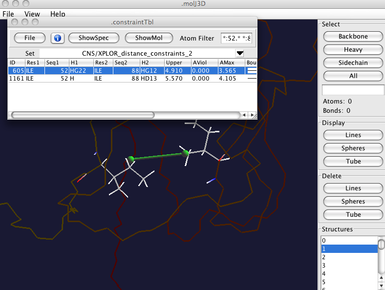
If you have the premium version of NMRVIEW with the crescent molecular viewer active then clicking the ShowMolbutton will display the atoms as shown here. The backbone will be shown somewhat dimmed, the bonds in each of the two residues involved in the constraint will be displayed, and a green connector drawn between the two highlighted atoms.

Constraint Map

The residue-residue pattern of constraints is displayed in a map colored by the number of restraints between that residue pair. You can display this map by selecting the File > Restraint Map menu item from the menu bar of the Constraint Table. Clicking on an item in the map will filter the constraint table to show all constraints involving that pair of residues If you have the premium version of NMRVIEW with the Crescent molecular viewer active then you will also see the molecule displayed with backbone as a tube, and lines connecting all residues involved in constraints as shown here.

Constraint Export/Import

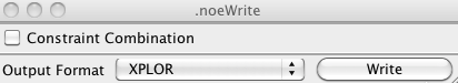
The general goal of constraint generation is to obtain a file of constraints that can be used in one of several structure calculation program. You can export the restraints displayed in the table to appropriately formatted files. Select the <span class="menuchoice">File > Write Constraints... menu item from the menu bar of the Constraint Table to get the following dialog. There are two items to select in the dialog. One is the format of the constraint file, which can be that used by XPLOR or that used by CYANA. The other is whether or not to use Constraint Combination. This is a method used within the CYANA program. By providing a similar capability here one can generate constraint files that already have combined constraints and use the appropriately formatted one in CYANA or XPLOR. Constraint combination is a way to minimize the effect of erroneous assignments. It works because if an erroneous constraint is combined into an ambiguous constraint with a valid constraint the erroneous constraint will have little impact on the calculated structure. If you randomly combine constraints, and a minority of them are erroneous it is likely that most of the erroneous constraints will be found in combination with a valid constraint. Having selected the two output options, click the Write button. A File Dialog will appear in which you can select the output file name.

Constraints can also be imported from the files formatted for XPLOR and the output files of ARIA. Use the File > Read XPLOR Constraints menu item of the Constraint Table to read XPLOR distance constraints. Use the File > Read ARIA XML Output menu item of the Constraint Table to read the output of an ARIA run. In both cases you will be prompted for the file to open.