Rate Analysis

The Rate analysis system is designed to facilitate the analysis of time dependent NMR properties. It can be used, for example, to extract relaxation rates or to visualize NOE build up curves. The procedure is used to analyze the intensities in a series of spectra collected with different mixing times. The analysis proceeds in a series of steps as follows:

1. Peak pick the spectrum with highest intensities.

2. Clean up peak lists.

3. Open the Rate Analysis Panel.

4. Set appropriate analysis parameters.

5. Analyze each peak in list.

Peak pick spectrum with highest intensities.

Choose one spectrum to peak pick. For relaxation analysis this is typically the spectrum with shortest mixing time. For NOE buildup curves it is typically one with an intermediate mixing time.

Clean up peaks

This step is not necessary, but it is useful to eliminate artifactual peaks at this stage. This is particularly relevant if all peaks are to be automatically analyzed. Any of the peak tools can be used for this step.

Open the Rate Analysis Panel.

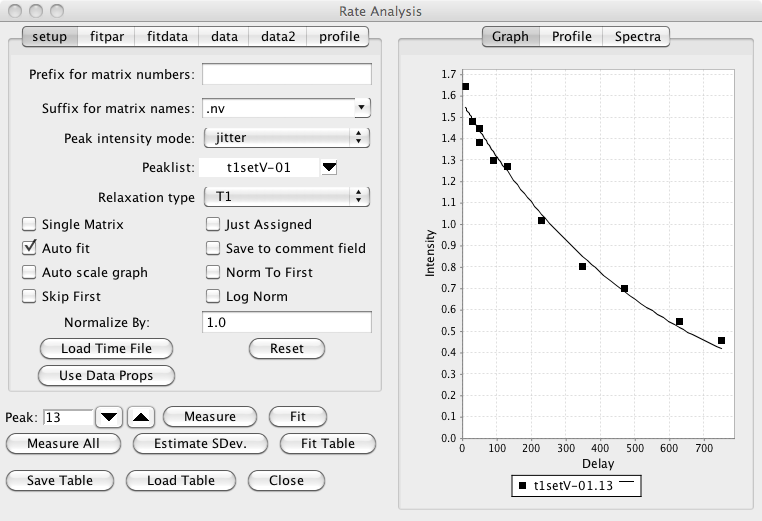
Choose "Rate Analysis" from the Analysis Menu of the NMRView Control Panel. The following analysis panel will appear.

Set appropriate analysis parameters.

Matrix Prefix

Sometimes you'll have a series of 2D spectra whose names can be decomposed into a prefix common to all spectra, and a unique descriptor for each spectrum. For example, T1_1.nv, T1_2.nv, T1_3.nv ..., or noe_0, noe_20, noe_40, ..., or T2a, T2b, T2c ... There is no requirement that the descriptors be numeric, or that the spectra be collected or numbered in any particular order. The prefix (T1_, T2, or noe_ in the above examples) should be entered into the field labeled "Matrix Prefix". It is necessary that the data files be named this way if you name are going to store the relaxation time into the dataset parameter file. If you are going to use a "Time File" you can leave this blank.

Matrix Suffix

The suffix for the matrices described above. For example, if the matrices are T1_1.nv, T1_2.nv, T1_3.nv, you would enter nv for the matrix suffix.

Intensity analysis mode

The estimation of the intensity of the peaks uses the "nv_peak analysis" command. This command returns various estimates of the peak intensity, including both peak height and peak volume values. The desired estimator type should be selected with the "Mode" menu. The default mode (Jitter) determines the height of the most intense point found within a certain range (+/- 25 % of the peak bounds) of the peak center. This allows for a certain level of variation of the peak position (i.e. jitter) from one spectrum to the next.

PeakList

The appropriate peak list (created in the step above) should be selected from the peak list menu.

Descriptor/Time File

A file must be created containing the unique descriptor portions of the file names and the corresponding mixing times. The file should have the a format where the each row corresponds to one dataset. The first column of the file contains a descriptor of the file and the second column contains the relaxation time. If you entered a value in the "Prefix for matrix numbers" field discussed above, then the descriptor is the part of the file name after the prefix. If you didn't enter any prefix, then use the whole file name (except for the file extension). For example: 1 20 2 100 3 60 4 200 5 50 6 140 Times should be entered in ms. The file can have any unique name.

Relaxation Type

This is used when saving data to a STAR save frame or peak comment field, and has no effect on the actual analysis process.

Single Matrix

The data to be analyzed can either be in individual datasets, or individual planes of a single pseudo-3D matrix. In the latter situation check this box. Then the description column of the Time File will be assumed to represent the plane number of the 3D matrix to be analyzed for relaxation time specified on that row of the file.

Just assigned

When automatically analyzing all peaks (see Measure All below), only peaks that have assignment values in their label fields will be included.

Auto fit

If checked, the non-linear regression analysis will be done each time you step to a new peak.

Save to comment field

Each peak as a comment field that can contain any string of text. If this check box is selected, then after each peak is analyzed its comment field will be set to contain the calculated relaxation rate.

Auto scale graph

Not currently used.

Norm to first

It is sometimes useful to normalize the measured intensities to the first value in a series. This is commonly done, for example, with the Relaxation-Dispersion analysis of CPMG datasets. Clicking this check box will divide each value in the series of data points measured for each peak by the first value in the series (hence the first value will now become 1.0).

Skip First

In some circumstances, for example analysis of Relaxation-Dispersion datasets, where the data is normalized by the first data point in the series, it is generally appropriate to exclude the first data point from the subsequent analysis. This data point may not for example, really be part of the relaxation series, but instead is a reference value. Clicking this check box will exclude the first data point from subsequent analysis.

Log Norm

If normalization (as described above) is done, it may also be appropriate to take the logarithm of the normalized values (typically this is done to convert the normalized values into a relaxation rate). Note, in some respects this log normalization may be considered to have adverse effects on the quality of the data fitting. This is because standard fitting algorithms presume that the errors in the experimental measurements are normally distributed. After taking the logarithm of the data this is not the case. When doing analysis of Relaxation-Dispersion experiments to calculate exchange rates there are two available equations (within NMRViewJ) that can be fit. If log-normalization is done you should use RDispSin, otherwise (and this author thinks that this is probably statistically more valid) you should use RDispESin.

Normalize by:

If normalization is done, as described above, you can also enter an explicit normalization value that will be included in addition to the normalization to the first data point.

Having setup the above parameters you can now load the relaxation delays. This can be done by either loading values stored in the relaxation delay file (as described above), or by extracting delay times from a delay parameter stored in each datasets parameter (.par) file.

Load Time File

When the user clicks this button a File Open dialog will appear. The user should select the previously created Descriptor/Time file. The file will be read, the descriptor and time data will be displayed in the data table, and the appropriate datasets will be automatically opened if they have not been previously opened.

Use Data Props

When the user clicks this button the names of any opened datasets will be scanned to find those that start with the specified prefix. The relaxation delay will be taken from the delay property specified for each dataset.

Reset

When the user clicks this button the relaxation information (delays) will be cleared.

Once the above parameters have been set, and the data loaded from the Time file, or dataset properties, you can use step through the peaks in the list using the up/down arrows next to the Peak entry. You can jump directly to an individual peak by typing its peak number into the peak entry and hitting the Enter key. As you step through each peak the intensity (or volume etc, as specified with the "Peak intensity mode") will be measured at the position of that peak in each of the datasets. The graph will be updated to show these intensity values as a function of the relaxation delay.

You can also observe each of the individual spectral peaks that are being quantified by choosing the "Spectra" tab (rather than the Graph tab) on the right hand side of the Rate Analysis interface. You may need to use the zoom in/out and scale up/down buttons on the icon bar to set the appropriate spectral display width and contour level.

Before actually performing a least squares fit of the data to determine the relaxation rate from the data you need to check several parameters in the fitpar tab.

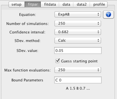
Equation

Choose an equation appropriate to the experiment used to collect the data. An important decision is whether to use a two or three parameter fit. The three parameter fit, which includes a parameter to estimate the intensity at infinite time, might be considered by some to be the most appropriate mode. Unless, however, the data has very low noise, and long mixing times are included in the experimental data the two parameter fit, which assumes the value at long mixing times, often gives the most reasonable estimate of the amplitude and rate parameters. It is, of course, up to the user to select and justify the most appropriate equation.

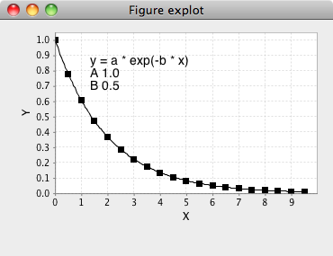
Equations are chosen from the "combobox" labeled Equation. To see the actual equation and a plot of it over a typical data range click the ? icon next to the equation chooser.

Confidence interval

Select a probability level to be used for the estimate of the confidence intervals of the fitted parameters. The confidence intervals are estimated using a Monte Carlo procedure.

Number of simulations

Select the number of simulations to be used in the Monte Carlo estimate of confidence intervals. There is no reason other than speed not to use a high value.

SDev. method

The Monte Carlo procedure used to estimate the confidence intervals of the fitted parameters requires and estimate of the standard deviation of the data intensities. This can be done in two ways. Either you can choose the Calc. method or use the Set method and explicitly set a value. The Calc method could be considered cheating, though can give a reasonable estimate. In this protocol, you fit the data, and use the root mean square value of the deviations of the measured values from the calculated values as an estimate of the standard deviation. This process happens automatically if you set the SDev method choice to Calc.

Alternatively you can explicitly enter a value in the Sev. value field and set the SDev. method to "Set". The value you enter could be taken from the analysis of the noise in a peak free region of the spectrum, or as is commonly done, from intensity values measured at a relaxation time that is replicated.

Analyze the peaks.

The peak to be analyzed can be selected by entering a peak number in the Peak field, or by using the up/down buttons to navigate through the list. As each peak is selected, the peak intensities for that peak will be extracted from each dataset and displayed in the XY plot window. The spectrum window will show an expansion of the spectrum region containing the peak. The dataset used for the spectrum display can be changed by selecting the check button next to the appropriate entry in the data table.

The intensity measured for each peak will also displayed as a table in the "data" tab. The first column is the dataset descriptor, the second column is the relaxation time for that dataset, and the third column is the measured intensity (as defined by the Peak intensity mode). The Norm to First and Log Norm modes will affect the measurement process and the values displayed in the table will reflect the state they were in when the datasets are analyzed.

Measure

Click this button to measure the intensities for the current peak. This is not normally necessary as intensities are automatically measured each time you step to a new peak. You might want to use it if you are checking the effect of changing the Peak intensity mode. Each time you change it click the Measure button to view the graph of the intensities calculated with the new mode.

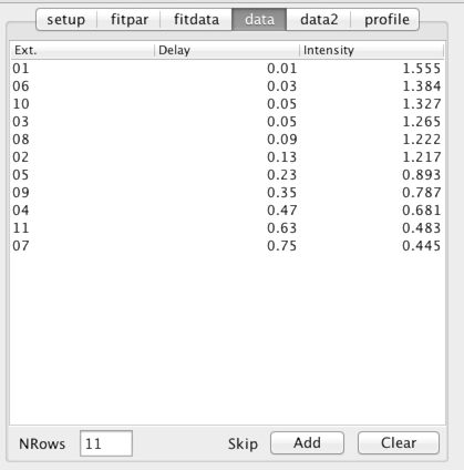
NMR is a technique that can be subject to an occasional artifact which might significantly affect the intensity of peaks in the spectrum. Such peaks will have a marked influence on parameters derived in this analysis. In some cases it may be judicious to remove these peaks from the analysis. This can be done by selecting one or more rows in the above table and clicking the Add button. This will add the data points corresponding to the selected row and the current peak to a list of peaks to be skipped during peak measurement and fitting.

Fit

Click this button to perform the non-linear fit to the currently displayed data. Non-linear fitting procedures generally require a starting point (a guess, hopefully educated) for each parameter to be fit. If the Guess Starting Point mode is on (and this is the default), the fitting procedure will automatic determine a starting point. Each equation built in to NMRViewJ has some rules that it uses to formulate a guess for each parameter.

After fitting, either by clicking this button, or going to a new peak if the "Auto Fit" mode is selected, the table in the fitdata tab will be populated with the results of the non-linear, least squares, fitting procedure. Each row of the table will correspond to one parameter from the equation used to fit the data. The starting value (guess) is displayed in the second column of the table and the best fit value in the third.

After the fitting procedure is performed once to determine the best fit value for each parameter, it is repeated a number of times as specified by the "Number of Simulations" parameter. Each of these subsequent fits is done to a simulated data set that is generated using the best fit parameters in the chosen equation. Random noise with a Gaussian distribution and a standard deviation equal to that set in the SDev Value field is added to the simulated data before fitting.

This Monte Carlo method generates a set of values for each of the parameters in the equation. The values for each parameter are sorted, and then values that bracket the fraction of values specified by the confidence interval are determined. Strictly speaking, for equations with non-linear parameters, the interval corresponding to a given percentile can be asymmetrical about the best fit parameter. For example, if the best fit value is 100, 5% of the values might be below 95, and 5% of the values above 110. Thus the 90% confidence interval would be from 95 to 110. Because of this it is not really appropriate to report the error distribution as a single number (a standard deviation). But, for NMR data fit to exponential decays the deviation from symmetry is often not huge, and it seems customary to report values as the best fit parameter plus or minus a single standard deviation value. NMRViewJ generates a single number by taking the geometric mean of the upper and lower values of the 0.682 confidence interval.

The standard deviation and upper and lower values of the specified confidence interval are displayed in the third,fourth and fifth columns of the table. The RMSD value (deviation of the data points calculated using the best fit parameters to the measured parameters) is displayed at the bottom of the table.

Measure All

Click this button to loop over all the peaks in the specified list and measure the intensity at the corresponding position in each of the datasets.

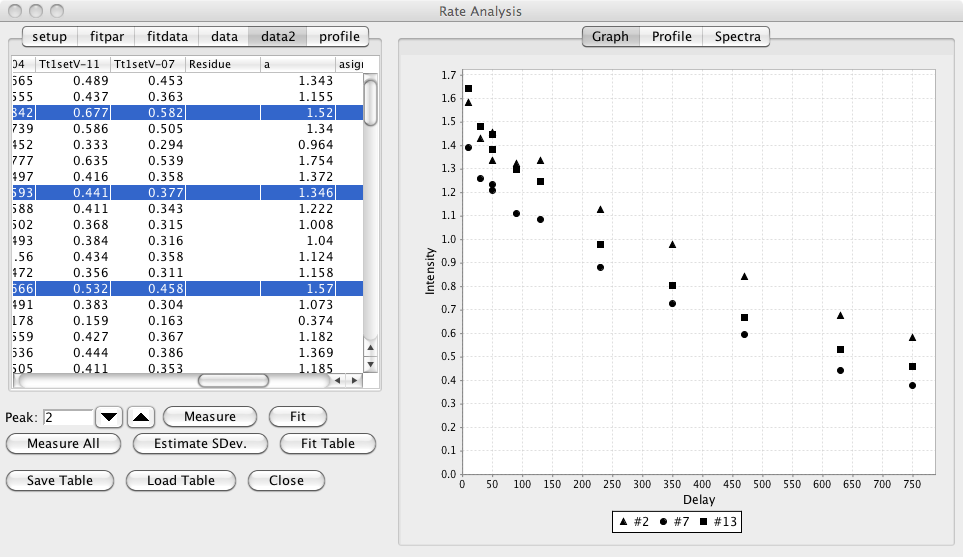
The table in the tab labeled data2 will now be populated with the measured data. The first column will contain the peak number and the second column will contain the number of datasets analyzed for each peak (this will be the same for every peak). The remaining columns will contain the intensity measured in each dataset (the column header will indicate the corresponding dataset descriptor).

Estimate Standard Deviation

A common protocol for estimating the standard deviation to be used in the Monte Carlo analysis depends on collecting two data sets at the same relaxation time. From the distribution of deviations between the intensities for each peak, in the two data sets, one can estimate the standard deviation.

Click this button to check the list of relaxation times for a replicate pair, If found, the standard deviation will be calculated and the entry in the "fitpar" tab will be updated with the value. You must have done the "Measure All" command prior to using this command.

Fit Table

Clicking this button will loop over the table of data generated with Measure All, and perform the non-linear least squares, fit on the data in each row. After fitting, additional columns will appear in the data2 table. A pair of columns will be present for each parameters best fit and standard deviation values. The last column will display the rmsd value for the fit. Additionally there will be one column (just before the best fit values) that will contain the residue number for the peak. This will only be populated with a value if the peak has an assignment label in the standard NMRViewJ format (residue.atomName).

Highlighting any rows (contiguous or non-contiguous) in the table will update the graph with the data values measured values and best fit lines (bug, line not showing).

Save Table

You can save the table of measured data (and best fit values if you've done the fitting) by clicking this button. You will be prompted for a file name in which to store the data. This provides a convenient way to export the data to be fit or displayed in some other application.

Load Table

You can reload a saved table of measured data (and best fit values if you've done the fitting) by clicking this button. You will be prompted for a file name from which to retrieve the data.

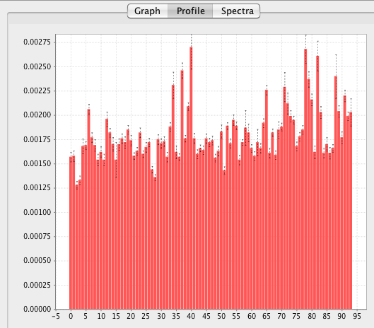
Having measured the data you might want to plot all the relaxation rates as a function of peak or residue number (if the peaks were assigned). This can be done by going to the Profile tab and selecting either Peak or Sequence mode and clicking the Display button. The Profile tab at the right side of the Rate Analysis interface will now show a bar chart (with indicators of the standard deviations) for all the relaxation rates (assumed to be the "b" parameter) in the data2 table.