Titration Analysis

The Titration analysis system is designed to facilitate the analysis of ligand dependent NMR properties. It can be used, for example, to extract binding constants or to visualize titration curves. The procedure is used to analyze the chemical shift positions of peaks in a series of spectra collected with different ligand concentrations. The analysis proceeds in a series of steps as follows:

1. Prepare spectra and concentration information.

2. Peak pick all the relevant spectra.

3. Clean up peak lists.

4. Open the Titration Analysis Panel.

5. Set appropriate analysis parameters.

6. Analyze relevant peaks (those that show ligand dependent shifts).

Ideally, you're spectra will be stored in a single directory with each file ending in a unique integer. So you might have files named titration1.nv titration2.nv, etc. Open all spectra by using <span class="menuchoice">Datasets > Open Datasets....

The concentration of ligand that is associated with each dataset can be stored either in each dataset's parameter (.par) file, or all the values can be stored in a single text file. If you want to store them in the parameter file, you'll need to ensure that you have parameter files for each dataset. Open the Datasets Table (<span class="menuchoice">Datasets > Dataset Table....), select all the datasets and click the WritePar button. This will save a ".par" file for each spectra (in the same directory as the ".nv" files). Manually edit each ".par" file to add a "property ligcon" line that specifies the ligand concentration for that file. You can also add a "property protcon" line the specifies the protein concentration for each dataset. This is useful, because often as you titrate in ligand to a sample you are also diluting the sample so the protein concentration is not the same for each file. Concentrations can be specified in any units, as long as you are consistent in all files, and use the same units for ligand and protein concentrations.

A typical parameter file will look like (with concentrations in micro-molar):

                dim 2 512 256 64 64
                sw 1 3940.88647461
                sf 1 499.718994141
                label 1 H1
                complex 1 0
                sw 2 1320.0
                sf 2 50.641998291
                label 2 N15
                complex 2 0
                posneg 1
                lvl 0.1
                scale 1.0e6
                rdims 0
                datatype 0
                poscolor black
                negcolor red
                ref 1 4.77299976349 513.0
                ref 2 120.01499939 109.0
                property ligcon 750
                property protcon 100

Now, reload the parameter files by selecting them in the Datasets Table and clicking the "ReadPar" button. Change the Datasets Table mode to Properties. You should now see a ligcon property (and protcon property if you entered it) for each file, with the appropriate value listed.

Alternatively, you can specify a single text file containing the information. The file has a single row for each dataset, with two or three fields per row. The first field is always the unique portion of the dataset file name. In this example the files were titr0000.nv, titr0050.nv, titr0100.nv etc. If you have not followed this naming scheme, with a common name portion (here titr) and a unique portion (0000, 0050 etc.) then you can simply specify the entire filename (without the ".nv" extension). The second field is the ligand concentration, and the third field (if present) is the protein concentration.

               0000 0.0 204
               0050 50 204
               0100 100 204
               0200 200 204
               0350 350 204
               0500 500 204
               0750 750 204
               1000 1000 234

This is most easily done by opening all the spectra in one window. To do this, select all the titration spectra in the Datasets Table and then click the "Draw" button. In the "Window Add" dialog that appears, change both the Rows and Columns values to "1" and click the "Create" button (if you don't change the Rows and Columns numbers each spectrum will appear in a separate gridded window). A window should appear with all the spectra displayed in it. It is very useful when displaying the spectra if they are colored in a sequential fashion, with colors starting at one value for low ligand concentrations, and blending into a different color for the high ligand concentration. You can easily do this by clicking the color gradient button on the Spectrum Attributes File Tab and choose one of the sequential color schemes. At this point you should also check the contour levels for the spectra and adjust them to a point where you think that if you peak pick the data you'll get, as much as possible, one peak for titrating nucleus for each dataset in the titration. Having set up the colors and contour levels, you again save the parameter files with this information. Just click the Save icon located on the File tab below the gradient icon.

Put the crosshair cursors around the spectral region you wish to pick and choose "Pick" from the Spectrum Menu's Peak submenu. This will pick all the spectra displayed in the window within the regions of the crosshairs. Each peak list will have a name corresponding to the dataset (titr0000 for dataset titr0000.nv etc.). You can also do this from the PeakPick tab of the Spectrum Attributes menu. Leave the peak list entry empty so each list will automatically pick up the name of the dataset. Note, at present the titration tool assumes that this mapping of peak list names to dataset names holds true. If not, because you created your peak lists in some other manner, it may not be able identify the appropriate peak lists, and you'll get an error about "Need to pick peaks first".

Now that you've picked peaks you might want to examine the spectrum again to double check the appropriateness of your contour level selection. You may want to change it and re-pick the peaks. If you change the contour level, then you should click the Save icon located on the File tab below the gradient icon again to save the parameter files with the new contour level.

Choose the Analysis > Titration Analysis menu item and the following analysis panel will appear.

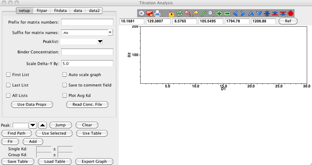
Various parameters effect how the titration analysis proceeds. In this step you'll set a series of parameters specified in the setup section of the Titration interface.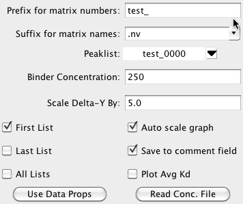

Prefix for matrix numbers

The analysis system typically assumes the the datasets consist of a series of 2D spectra whose names can be decomposed into a prefix common to all spectra, and a unique descriptor for each spectrum. For example, ligand_1.nv, ligand_2.nv, ligand_3.nv. There is no requirement that the descriptors be numeric, or that the spectra be collected or numbered in any particular order. The prefix (ligand_ in the above examples) should be entered into the field labeled "Matrix Prefix". If you are using a single text file to store the concentration data, and the first field of that file contains the complete file name, then leave the Prefix field empty.

Matrix Suffix

The suffix for the matrices described above. For example, if the matrices are ligand_1.nv, ligand_2.nv, ligand_3.nv, you would enter nv for the matrix suffix.

PeakList

The peaklist corresponding to the lowest ligand concentration should be selected from the peak list menu.

Binder Concentration

The standard equation used for binding analysis as a parameter for the concentration of the molecule that the ligand is binding to. Enter the concentration of that molecule here. The concentration should be expressed in the same units as that used for the ligand concentration specified in the spectrum parameter files. This value will only be used if you did not specify a binder concentration along with the ligand concentration for each dataset.

Scale Delta-Y By

When the titration tool measures the chemical shift change of the peaks from one ligand concentration to another it uses a combination of the chemical shift change (expressed in PPM) in each of the two dimensions (typically hydrogen and nitrogen). Because nitrogen resonances shift over a larger chemical shift range than protons, if one weighted the change in the two dimensions equally, nitrogen shifts would disproportionately effect the combined shift value. Accordingly it is common to scale down the shifts in one dimension. The default value used is 5.0, but some users will wish to use different values. For example, some researches prefer 10.0 as that is the ratio of the magnetogyric ratios for hydrogen and nitrogen. The default value was set to 5.0 as that is approximately the ratio of the standard deviation of the the linewidths (in ppm) of the nitrogen and hydrogen peaks, and thereby scales the data relative to the uncertainty in the peak positions.

First List

As you move from peak to peak the spectrum will be updated to show the region around the current peak. Peak boxes for the peaks will optionally be displayed as well. It may be too cluttered to see all peaks. Click this checkbutton on to display the peaks corresponding to the lowest ligand concentration.

Last List

Click this checkbutton on to display the peaks corresponding to the highest ligand concentration.

All Lists

Click this checkbutton on to display the peaks corresponding to all ligand concentrations.

Auto Scale

Click this checkbutton on so that the XY titration graph is automatically scaled each time you move to a new peak. Having it off makes it easier to tell the absolute value of the shift changes.

Save to comment

Each peak has a field available for comments. If this checkbutton is turned on, then each time you fit a peak the measured Kd will be stored in the peaks comment field.

Plot Avg Kd

Ideally, when measuring the Kd for some phenomenon you will be fitting peaks that all are titrating with the same Kd. When you multiple titration curves in this tool you have the choice of plotting each curve with its own best fit Kd, or plotting them all with the average Kd. This is a very qualitative measure, but if the fits look significantly worse with the average Kd it is likely that multiple binding phenomena are occurring and you are measuring contributions with distinct Kd values.

Your choice here will depend on whether you stored the concentration data in individual parameter files for each dataset, or in a single text file.

Use Data Props

When the user clicks on the "Use Data Props" the ligand concentrations associated with each spectrum will be loaded and various variables used in the analysis will be initialized.

Read Conc. File

When the user clicks on the "Use Data Props" the ligand concentrations associated with each spectrum will be loaded and various variables used in the analysis will be initialized.

Equation

Choose an equation appropriate to the experiment used to collect the data. At present, the relevant equation in the titration analysis tool is Quadratic10: A+(C-A)*((Pt+x+10\^B)-((Pt+x+10\^B)\^2 - 4Pt*x)\^0.5))/(2*Pt) The parameters for this equation are: A, the chemical shift difference at zero concentration, B, the logarithm (base 10) of the dissociation constant, C, the chemical shift difference at infinite concentration. Pt, in this equation, will be replaced with the "Binder Concentration" described above.

Note carefully that the fitted B value corresponds to the logarithm of the dissociation constant. For example, if the best fit value is -3.0, and the concentrations have been entered in Molar concentration units, the dissociation constant is 1.0 mM. There are a variety of reasons why the fit is done this way. For example, this ensures that it is impossible to end up with a dissociation constant that is negative (a physical impossibility). If you prefer to not fit this way, use the Quadratic equation.

Confidence interval

Select a probability level to be used for the estimate of the confidence intervals of the fitted parameters. The confidence intervals are estimated using a Monte Carlo procedure.

Number of simulations

Select the number of simulations to be used in the Monte Carlo estimate of confidence intervals. There is no reason other than speed not to use the a large value.

SDev. Method

Proper estimation of the uncertainty of the fitted parameters by the Monte Carlo method requires an estimate of the uncertainty of the chemical shift positions. There are two supported methods for doing this. First, setting SDev. Method to Calc, will fit the data to the specified equation, then estimate the standard deviation from the deviations of the original data points to the fitted values. The alternative is to set the Method to Set, and enter a specific value into the SDev. value field. One method to estimate the standard deviation value to enter here would be to measure the average line width of the peaks, as this provides an estimate of the uncertainty of the peak positions.

Bound Parameters

The equation used in the titration analysis has a parameter A which defines the peak movement at 0.0 ligand concentration. You might want to hold this parameter fixed at 0.0. Just enter "A 0" into the Bound Parameters field. You can of course enter different or additional parameters to be fixed to specified values.

The peak to be analyzed can be selected by entering a peak number in the Peak field, or by using the up/down buttons to navigate through the list. As each peak is selected the region around that peak will be displayed in the Titration Analysis tool's spectrum window. You may need, at this point, to adjust the spectrum view, zooming in or out depending on how large the shift of titrating peaks are, and also adjust the vertical scaling for a good view. Selecting the "First List" checkbutton will generally make the display easier to see and tell which peak corresponds to the first point in the titration. When you move to each peak the current peak will be selected (shown with a filled yellow footprint).

You can also jump to a specific peak displayed in the spectrum. Click on the peak in the spectrum, and then click the Jump button. The peak number will be set to that of the selected peak and the display will center on it.

Once the peak is selected there are three methods to extract the shift values to be used in the fit. Each time you load the data with the first two methods, the table in the data pane will be updated with the actual titration shift values.

Find Path

Click this button to automatically find a series of peaks that are presumably derived from the same atom. The search starts at the first peak and then searches outward, testing various possible "paths" through nearby peaks to find the one with the best linearity.

The path through the peaks will be highlighted with a green arrow on the spectrum. The arrows (all of them) can be cleared by clicking Clear.

Use Selected

When a titrating residue crosses paths with another residue, NvJ can get confused and choose a bad path (using Find Path to automatically follow the titration) To correct the path, zoom into residue closely . Ensure that the "All Lists" checkbox is selected in the Titration Analysis setup tab and that the cursor is in Select mode (choose Cursor-Select) from the spectrum's pop-up menu (it should default to this mode, in the Titration Analysis spectrum). Holding the shift key down, manually select peaks in the titration. You can also press the shift key down and drag the cursor across the set of peaks you desire to be selected. The order in which you select peaks doesn't matter. One you've selected the peaks corresponding to the titration of a single residue, click on Use Selected to load the titration shift values for the selected peaks. If you accidentally choose a peak from the other residue’s peak list, you will get an error message.

Use Table

It is also possible to manually type values into the table present on the "data" tab. Type new values into the table, hitting the Return key, after entering a value, and then click the "Use Table" button. You should see the graph update to reflect the new values in the table.

Fit

Click this button to perform the non-linear fit to the currently displayed data.

The best fit, standard deviation, and the minimum and maximum values for the specified confidence level will be displayed in the "fitdata" tab. The Kd measured for the currently fitted data, and the standard deviation will be displayed below the Fit button on the row labeled "Single Kd:". Note that even if the best fit parameter is log(Kd), the value displayed here will be the actual Kd.

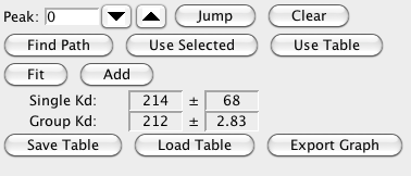
Add

Each time you fit the data for a different residue you can add the fitted data to the data2 table. Each row of the table will show the Kd, its standard deviation, the actual best fit A, B and C parameters, and the actual concentration and chemical shift data that was used in the fit. The Group Kd: display area will show the average Kd of all the values in the data2 table if now rows are selected, or the average of the values in any selected rows.

The best fit, standard deviation, and the minimum and maximum values for the specified confidence level will be displayed in the "fitdata" tab.

You can titration curves for data loaded into the data2 table. Just highlight one or more rows and the corresponding plots will appear in the chart

.

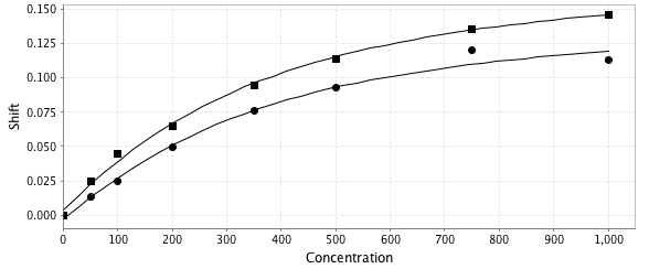Save Table

All the data in the data2 table can be saved by clicking this button. The saved text file can be a useful resource if you wish to do data fitting in some other program or reload a project.

Load Table

Click this to reload a table of saved data.

Export Graph

Click this to export the titration graph into a a graphical file.